An Overview of EE5731 Visual Computing

09 May 2021 in Modules Memo📝 2022-12-08

Visual Computing is a module I took this semester at NUS ECE, hosted by Assoc. Prof. Robby Tan. It covers some of the best-known classic CV algorithms.

These years, rapid progressions in Deep Learning have brought enormous improvements to vision-based applications. DL methods, mainly based on CNN frameworks, are constructed usually by training instead of the domain-specific designing and programming in the traditional CV algorithms. They are easy to build, often achieve better accuracy, and the trained models can be very lightweight. So why do we still need to learn about traditional CV methods?

EE5731 - Depth Estimation from Stereo and Video

06 May 2021 in Modules Memo📝 on Modules 2022-12-08

The second assignment of Visual Computing.

EE5731 - Panoramic Image Stitching

04 May 2021 in Modules Memo📝 on Modules 2022-12-08

SIFT is an algorithm from the paper Distinctive Image Features from Scale-Invariant Keypoints, published by David G. Lowe in 2004. The solution for one of its application, image stitching, is proposed in Automatic Panoramic Image Stitching using Invariant Features, by Matthew Brown and David G. Lowe in 2017. The continuous assessment 1 of Visual Computing is based on these two papers.

EE5731 - Viola-Jones Face Detection Algorithm

03 May 2021 in Modules Memo📝 2022-12-08

Viola-Jones algorithm is proposed on ICCV 2001 by, of course, Paul Viola and Michael Jones. Details and explanations of this algorithm can be found everywhere, and the module EE5731 also gives you step-by-step instructions. Even so, I would love to review the algorithm again for two reasons: It’s a good start for the millennials to have a view of CV 20 years ago. Also, there are some fun facts about the algorithm that are not covered in the lessons.

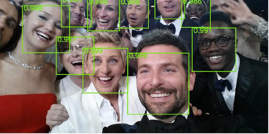
1. Viola-Jones Face Detection Algorithm

1. Viola-Jones Face Detection Algorithm

Face detection or object detection is a binary classification problem different from face recognition. Face detection can consider a substantial part of face recognition operations. Opposite to many of the existing algorithms using one single strong classifier, the Viola-Jones algorithm uses a set of weak classifiers, constructed by thresholding each of the Haar-like features. They can then be ranked and organized into a cascade.

The 3 main contributions in Viola-Jones face detection algorithm are integral image, AdaBoost-based learning and cascade classifier structure. The first step is to apply Haar-like feature extraction, which is an accelerated variant of image convolution using integral image. The lengthy features are then being selected by a learning algorithm based on AdaBoost. The cascade classifiers can drop the negative samples quickly and expedite the testing process enormously. Let’s have a quick go through towards the important points of the paper.

1.1 Feature Extraction: Haar-like Features

We can format this step as:

Input: a 24 × 24 image with zero mean and unit variance
Output: a 162336 × 1 scalar vector with its feature index ranging from 1 to 162336

This paper is a good example of combining classical CV with ML techniques. In the feature extraction step, CNN is not used. Instead, the intuitive Haar-like features are adopted.

Figure 1

The sum of the pixels which lie within the black regions is subtracted from the sum of pixels in the white regions. The mask set consists of 2 two-rectangle edge features, 2 three-rectangle line features, and a four-rectangle feature, which can be seen as a diagonal line feature. They are called Haar-like since the elements are all +1/-1, just like the square-shaped functions in Haar wavelet.

They are effective for tasks like face detection. Regions like eye sockets and cheeks usually have a distinctly bright and dark boundary, while nose and mouse can be considered as lines with a specific width.

Figure 2

The masks are applied over the sliding windows with a size of 24x24. The window is called a detector in the paper and 24x24 is the base solution of the detector. We’ll discuss how to get the detectors later. The 5 masks, starting from size 2x1, 3x1, 1x2, 1x3, 2x2, to the size of a detector, will slide over the whole window. For example, a 2x1 edge mask will move row by row, then extend to 4x1 and move all over the window again … until 24x1; then it starts over from 2x2 to 24x2, 2x3 to 24x3, 2x4 to 24x4 … till it became 24x24.

It’s time to answer why the length of the output descriptor is 162,336. A 24x24 image has 43,200, 27,600, 43,200, 27,600 and 20,736 features of category (a), (b), (c), (d) and (e) respectively, hence 162336 features in all.

Here is a MATLAB script for the calculation of the total number of features. Note that some would say the total number is 180,625. That’s the result when you use two four-rectangle features instead of one.

frameSize = 24;
features = 5;
% All five feature types:
feature = [[2,1]; [1,2]; [3,1]; [1,3]; [2,2]];
count = 0;
% Each feature:
for ii = 1:features
    sizeX = feature(ii,1);
    sizeY = feature(ii,2);
    % Each position:
    for x = 0:frameSize-sizeX
        for y = 0:frameSize-sizeY
            % Each size fitting within the frameSize:
            for width = sizeX:sizeX:frameSize-x
                for height = sizeY:sizeY:frameSize-y
                    count=count+1;
                end
            end
        end
    end
end
display(count)

Now we understand how to define and extract our features. But some detailed operations are still not covered, which made me confused when I first learned this part of the algorithm.

⚠️ Nitty-gritty alert!

Getting Detectors
So where do the detectors come from? A video I found gives the perfect demonstration.
The size of a box that might have a face inside varies a lot between different photos. (The size of the original photos in the discussion is 384x288.) So basically we can select the size of the box empirically (no smaller than 24x24) and then resize it to a 24x24 detector.
The paper also proposed a standardized scheme. We can scan the image with a 24x24 fixed size detector. Instead of enlarging the detector, the image is down-sampled by a factor of 1.25 before being scanned again. A pyramid of up to 11 scales of the image is used, each 1.25 times smaller than the last.
The moving step of the 24x24 detector is one pixel, horizontally and vertically. For the resized image, the equivalent moving step is larger than 1. So the down-sampled image pyramid can adjust the equivalent detector size and the moving step size at the same time.

Normalization before Convolution
The selected 24x24 detectors are first normalized before the convolution with the features. If the variance of a detector is lower than a specific threshold, then it must be plain and has little information of interest which can be left out of consideration immediately, saving some time processing the backgrounds.

Performance Issue
In fact, for better detection performance we can discard 3 features and only keep features (c) and (b). Like in Figure 2. Given the computational efficiency, the detection process can be completed for an entire image at every scale at up to 15 fps. Of course, with advanced machines 20 years later it’s better to utilize all the 5 Harr-like features.

1.2 Fasten Convolution Process: Integral Image

Input: a N × M image I
Output: a N × M integral image II

Remember the +1/-1 rectangles in Haar-like features? It’ll be tedious if we simply multiply the feature masks with the pixels in the corresponding region. Integral image is a smart way to replace the convolution with only a few additions.

Figure 3

In an integral image, each pixel at $(x,y)$ is the sum of all the pixels on the top-left: $II(x,y) = \sum_{i=1}^{x} \sum_{j=1}^{y} I(i,j)$

This simplified representation with sums of rectangles can speed up the feature extraction significantly. Only $1+2+1+2+4=10$ operations are needed to compute the convolution of 5 masks on one position.

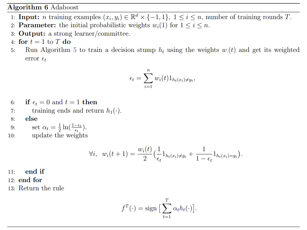
1.3 Feature Selection: AdaBoost

Input: the descriptor $x$ and label $y$ for each training sample (about 5k positive and 5k negative)
Output: a strong classifier $h(x)$ consists of $T$ weak classifiers $h_t(x)$ from $T$ features

This step is to train a classification function using the feature set (a set of Haar-like feature masks with different sizes, patterns, and locations all over the images) and a training set of positive and negative images (no less than 5,000 24x24 faces and 5,000 24x24 non-faces). The illustration below can help build a good understanding quickly.

Full-width image

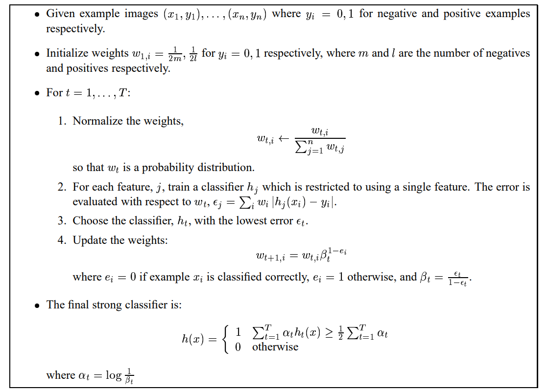
Figure 4 AdaBoost Algorithm

A weak classifier is chosen on each iteration. And the falsely classified samples are given higher weights in the next iteration. The next classifier will pay extra attention to the misclassified training samples. Combining the weak classifiers, in this case, the low-level boundaries, we have a high-level boundary, which is considered as a strong classifier.

People always describe AdaBoost as a Forest of Stumps. The analogy just tells the exact nature of AdaBoost. AdaBoost means Adaptive Boosting. There are many boosting algorithms. Remember the random forest binary classifier? Each of the trees is built with random samples and several features from the full dataset. Then the new sample is fed into each decision tree, being classified, and collect the labels to count the final result. During the training process, the order doesn’t matter at all, and all the trees are equal. In the forest of stumps, all the trees are 1-level, calling stumps (only root and 2 leaves in binary classification problems). Each stump is a weak classifier using only 1 feature from the extracted features. First, we find the best stump with the lowest error. It will suck. A weak classifier is only expected to function slightly better than randomly guessing. It may only classify the training data correctly 51% of the time. The next tree will then emphasize the misclassified samples and will be given a higher weight if the last tree doesn’t go well.

Figure 5

The algorithm from the paper can be summarized as above. It’s adequate for a basic implementation of the algorithm, like this project. Despite this, there are still some details that merit the discussion.

⚠️ Nitty-gritty alert!

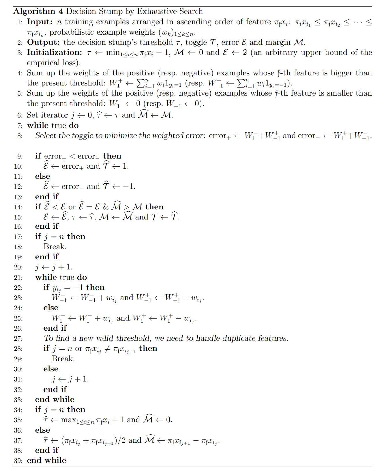
1.3.1 Decision Stump by Exhaustive Search

Input: the $f$ -th feature of all $n$ samples, the weights of all samples Output: a weak classifier $h_t(x)$

Now we know how to combine a series of weak classifiers to form a strong classifier. But the optimal decision stump search, that is, how to find the $h_j(x)$ in step 2 of the loop in AdaBoost algorithm shown in Figure 4, is always left out in some projects like this, and even in the paper itself.

Luckily, an explanation I found solved all my problems. The resources mentioned in this post are listed in the reference section.

A single decision stump is constructed with 4 parameters: threshold, toggle, error, and margin.

Parameter	Symbol	Definition
Threshold	$\tau$	The boundary of decision.
Toggle	$\Tau$	Decide if it means +1 (positive) or -1 (negative) when $>\tau$ .
Error	$\Epsilon$	The classification error after threshold and toggle are set up.
Margin	$\Mu$	The largest margin among the ascending feature values.

The exhaustive search algorithm of decision stumps takes the $f$ -th feature of all the $n$ training examples as input, and returns a decision stump’s 4-tuple $\left\{ \tau, \Tau, \Epsilon, \Mu \right\}$ .

First, since we need to compute the margin $\Mu$ , the gap between each pair of adjacent feature values, the $n$ examples are rearranged in ascending order of feature $f$ . For the $f$ -th feature, we have $x_{f_1} \leq x_{f_2} \leq x_{f_3} \leq ... \leq x_{f_n}$

$x_{f_n}$ is the largest value among the $f$ -th feature of all $n$ samples. It doesn’t mean the $n$ -th sample since they are sorted.

In the initialization step, $\tau$ is set to be smaller than the smallest feature value $x_{f_1}$ . Margin $\Mu$ is set to 0 and error $\Epsilon$ is set to an arbitrary number larger than the upper bound of the empirical loss.

Inside the $j$ -th iteration, a new threshold $\tau$ is computed, which is the mean of the adjacent values: $\hat{\tau} = \frac{x_{f_j} + x_{f_{j+1}}}{2}$

And the margin is computed as: $\hat{\Mu} = x_{f_{j+1}} - x_{f_j}$

We compute the error $\hat{\Epsilon}$ by collecting the weight $w_{f_j}$ of the misclassified samples. Since the toggle is not decided yet, we have to calculate $error_+$ and $error_-$ for both situations. If $error_+ < error_-$ , then we decide that toggle $\hat{\Tau} = +1$ , otherwise $\hat{\Tau} = -1$ . Finally, the tuple of parameters with smallest error is kept as $\left\{ \tau, \Tau, \Epsilon, \Mu \right\}$ .

Full-width image

Figure 6 Decision Stump by Exhaustive Search

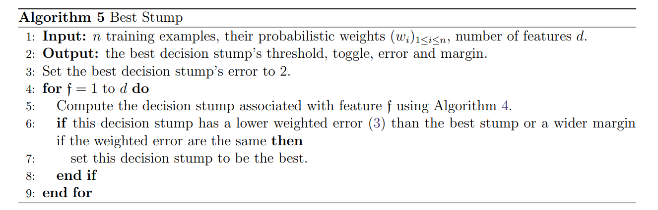
1.3.2 Selecting the Best Stump

Input: $d$ stumps for $d$ given features
Output: the best decision stump

During each training round $t$ in AdaBoost, a weak classifier $h_t(x)$ is selected. For each feature, we utilize the method in 1.3.1 to decide on the best parameter set for the decision stump.

$1 \leq t \leq T$ , $T$ is the total number of weak classifiers, usually we let $T$ be the full length of the feature vector.

The best stump among all the stumps should have the lowest error $\Epsilon$ . We select the one with the largest margin $\Mu$ when the errors happen to be the same. It then becomes the $t$ -th weak classifier. The weights assigned to all $n$ samples will be adjusted, and thus the exhaustive search should be carried out again using the updated weights. The idea behind this part is quite straightforward.

Full-width image

Figure 7 Best Stump

Full-width image

Figure 8 AdaBoost Algorithm with Optimal $h_t(x)$

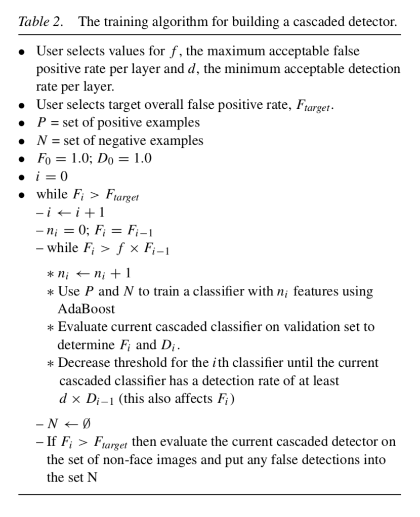
1.4 Fasten Classification: Cascade Classifier

Input: samples and features
Output: a cascade classifier, each step consists of several weak classifiers

As described in the subtitle, the main goal of building the cascade is to accelerate the estimation when dealing with a new input image, say, 384x288 (preset in the paper). Most of the sub-windows used to detect potential faces will have negative output. We hope to drop out those with backgrounds and non-faces as soon as possible.

Some will call this an attentional cascade. We hope to pay more attention to those sub-windows that might have faces inside them.

Our goal can be summarized as:

Weed out non-faces early on to reduce calculation.
Pay more attention to those hard samples since negative samples are dropped in advance.

Figure 9

The decision cascade is formed using a series of stages, each consists of several weak classifiers. Recall the strong classifier we build in 1.3, $h(x)$ is the sum of weighted votes of all the weak classifiers/stumps. This scheme is already sufficient to achieve face detection. Some projects just use this form of strong classifier instead of an attentional cascade. But the first goal reminds us that we shouldn’t use all $T$ weak classifiers to deal with every detector, which will be extremely time-consuming.

At each stage, or some may call it a layer or classifier, we can use only part of the weak classifiers, as long as a certain false positive rate and detection rate can be guaranteed. In the next stage, only the positive and false-positive samples (the hard samples) are used to train the classifier. All we need to do is set up the maximum acceptable false-positive rate and the minimum acceptable detection rate per layer, as well as the overall target false positive rate.

Figure 10

We iteratively add more features to train a layer so that we can achieve a higher detection rate and lower false-positive rate, till the requirements are satisfied. Then we move to the next layer. We obtain the final attentional cascade once the overall target false positive rate is low enough.

Hope my interpretation can help you understand the algorithm.

1.5 Additional Comments: AdaBoost in Paper Gestalt

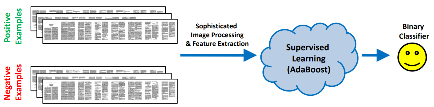
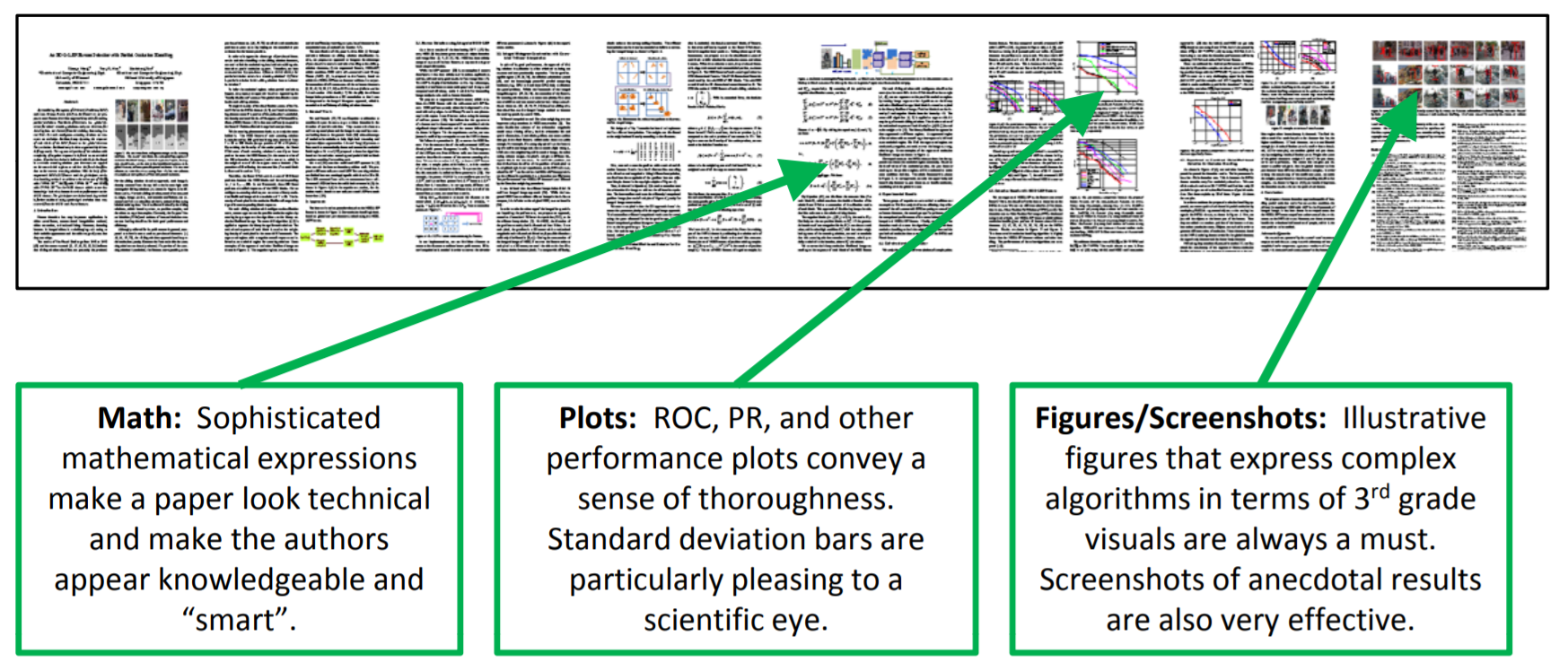
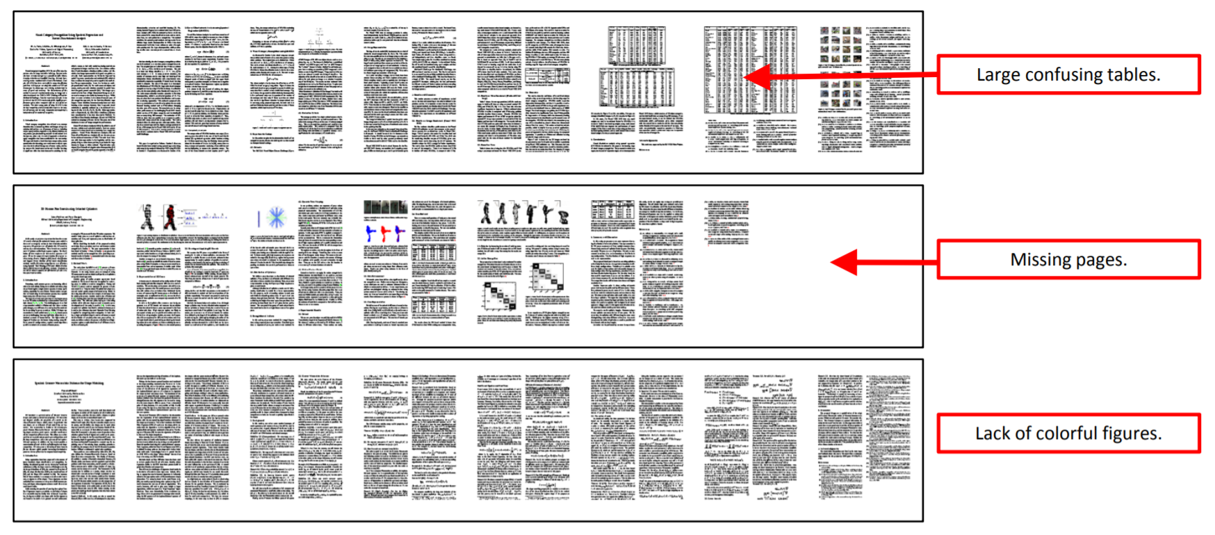
Laziness is the mother of invention. Some people, mostly the CVPR reviewers, are trying to use AdaBoost to classify bad papers from good ones just by judging the layout and formatting of them. The algorithm from the paper Paper Gestalt can achieve a true negative rate of over 50% with a false negative rate of about 15%. The classification of a paper needs only 0.5s.

Full-width image

Figure 11 Training Procedure of Paper Gestalt

It’s very entertaining and also educational since it gives some comments on the characteristics of good and bad papers. It’s funny that in order to be classified as a qualified paper for CVPR, the authors intentionally added a set of Maxwell’s equations to it. Weird but effective!

Full-width image

Figure 12 A Good Paper

Full-width image

Figure 13 A Bad Paper

1.6 Reference

Notes on Policy Gradient Methods

07 Feb 2021 in Projects 2022-12-08

Some notes on Chapter 13 - Policy Gradient Methods from Sutton & Barto’s book Reinforcement Learning: An Introduction in 2017.

1. The Framework of the RL Book
2. Notes on Policy Gradient Methods
- 2.1 What’s Policy Gradient?
- 2.1 Monte Carlo Policy Gradient and the Policy Gradient Theorem
  - 2.1.1 The Policy Gradient Theorem (episodic case)
  - 2.1.2 Monte Carlo Policy Gradient Algorithm

1. The Framework of the RL Book

The book Reinforcement Learning: An Introduction provides a clear and simple account of the key ideas and algorithms of reinforcement learning. The discussion ranges from the history of the field’s intellectual foundations to some of the most recent developments and applications. A rough roadmap is shown as follow. (Not exactly the same as the contents.)

Tabular Solution Methods
- A Single State Problem Example: Multi-armed Bandits
- General Problem Formulation: Finite Markov Decision Processes
- Solving Finite MDP Using:
  - Dynamic Programming
  - Monte Carlo Methods
  - Temporal-Difference Learning
- Combining:
  - MC Methods & TD Learning
  - DP & TD Learning
Approximate Solution Methods
- On-policy:
  - Value-based Methods
  - Policy-based Methods
- Off-policy Methods
- Eligibility Traces
- Policy Gradient Methods (we are here)

2. Notes on Policy Gradient Methods

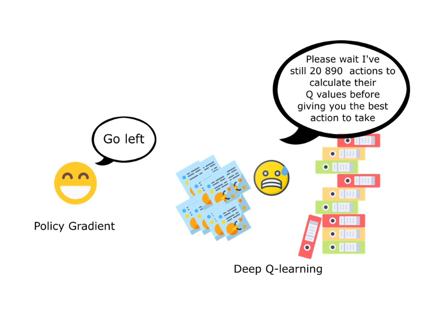
2.1 What’s Policy Gradient?

Almost all the methods in the book have been action-value methods until Chapter 13. In this chapter, a parameterized policy is learned, with or without learning a value function.

Policy Gradient is:

Methods that learn a parameterized policy that can select actions without consulting a value function.
The parameters are learned based on the gradient of some scalar performance measure J(θ) with respect to the policy parameter.
The general scheme of an update in policy gradient methods looks like this. It seeks to maximize performance.

\theta_{t+1} = \theta_t + \alpha \widehat{\nabla J(\theta_t)}

There might or might not be a learned value function. If both the approximations of policy and value function are learned, then it’s called an actor-critic method. (‘critic’ is usually a state-value function)
$\widehat{\nabla J(\theta_t)}$ is a stochastic estimate whose expectation approximates the gradient of the performance measure, with respect to its argument $\theta_t$ . This is an important rule that all the variants of policy gradient methods should follow:

E[\widehat{\nabla J(\theta_t)}] \approx \nabla J(\theta_t)

Why don’t we use the gradient of the performance $\nabla J(\theta_t)$ directly?
A proper selection of performance function is the state-value function $v_\pi (s)$ . Let’s define the performance measure as the value of the start state of the episode, $J(\theta) = v_{\pi_\theta}(s_0)$ . The performance is affected by the action selections as well as the distribution of states, both off which are functions of the policy parameter. It’s not hard to compute the effect of the policy parameter on the action and reward given a state. But the state distribution is actually a function of the environment and is typically unknown.

Note that the following discussion is for the episodic case with no discounting $(\gamma = 1)$ , without losing meaningful generality. The continuous case has almost the same property. The only difference is that if we accumulate rewards in the continuous case, we will finally get $J(\theta) = \infty$ . It’s meaningless to optimize an infinite measure.

2.1 Monte Carlo Policy Gradient and the Policy Gradient Theorem

Monte Carlo Policy Gradient, also called Vanilla Policy Gradient or REINFORCE, has a simple form given as: $\theta_{t+1} = \theta_t + \alpha \sum_a \hat{q}(S_t, a, \omega) \nabla \pi(a\vert S_t, \theta)$

$\hat{q}(S_t, a, \omega)$ is a learned approximation to $q_\pi(S_t, a)$ . It’s so called ‘critic’ and is parameterized by $\omega$ .

That is, we let $\widehat{\nabla J(\theta_t)} = \sum_a q_\pi(S_t, a) \nabla \pi(a\vert S_t, \theta)$ .

Recall the standard for a function to become a performance measure. Surely that this equation should be satisfied: $E[\sum_a q_\pi(S_t, a) \nabla \pi(a\vert S_t, \theta)] \approx \nabla J(\theta_t)$

or $E[\sum_a q_\pi(S_t, a) \nabla \pi(a\vert S_t, \theta)] \propto \nabla J(\theta_t)$

The proof of this is what the Policy Gradient Theorem is all about. The derivation is a lot of fun.

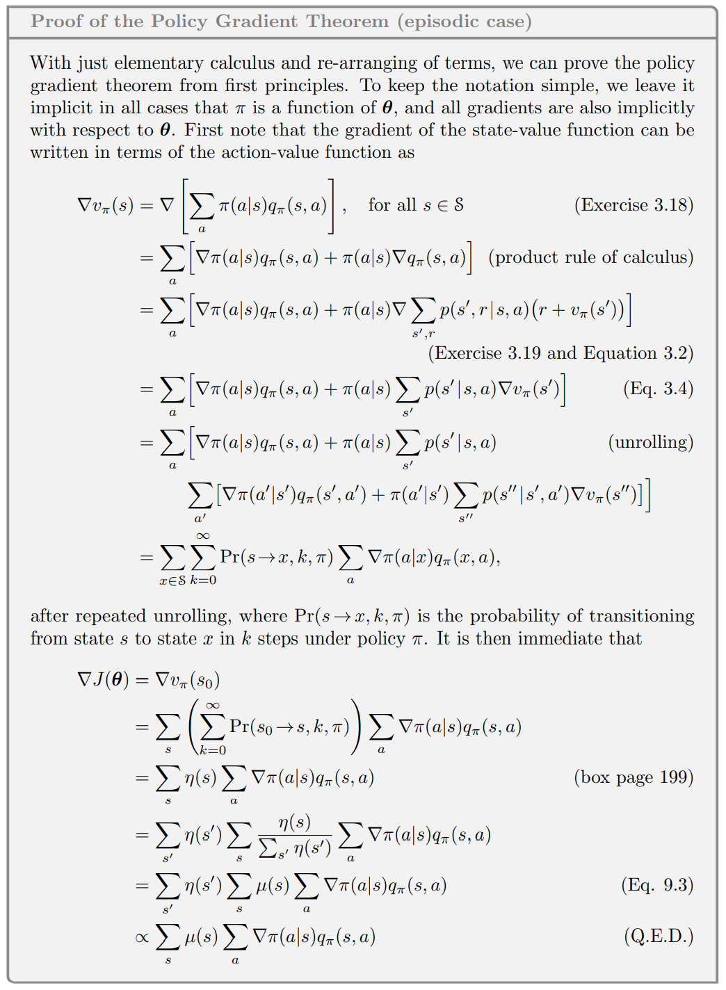
2.1.1 The Policy Gradient Theorem (episodic case)

Full-width image

Figure 1

Under construction $\begin{aligned} %!!15 \phi(x,y) &= \phi \left(\sum_{i=1}^n x_ie_i, \sum_{j=1}^n y_je_j \right) \\[2em] &= \sum_{i=1}^n \sum_{j=1}^n x_i y_j \phi(e_i, e_j) \\[2em] &= (x_1, \ldots, x_n) \left(\begin{array}{ccc} \phi(e_1, e_1) & \cdots & \phi(e_1, e_n) \\ \vdots & \ddots & \vdots \\ \phi(e_n, e_1) & \cdots & \phi(e_n, e_n) \end{array}\right) \left(\begin{array}{c} y_1 \\ \vdots \\ y_n \end{array}\right) \end{aligned}$

An optional caption for a math block

2.1.2 Monte Carlo Policy Gradient Algorithm

Under construction

Robust Real-time Object Detection (ICCV2001)

03 Dec 2020 in Weekly Papers📜 2021-03-09

Robust Real-time Object Detection on ICCV 2001 is proposed by Paul Viola and Michael Jones, which introduced a general framework for object detection. The paper, also named Robust Real-time Face Detection and Rapid Object Detection using a Boosted Cascade of Simple Features (on CVPR 2001), has over 15,000 citations.