EE5731 - Panoramic Image Stitching
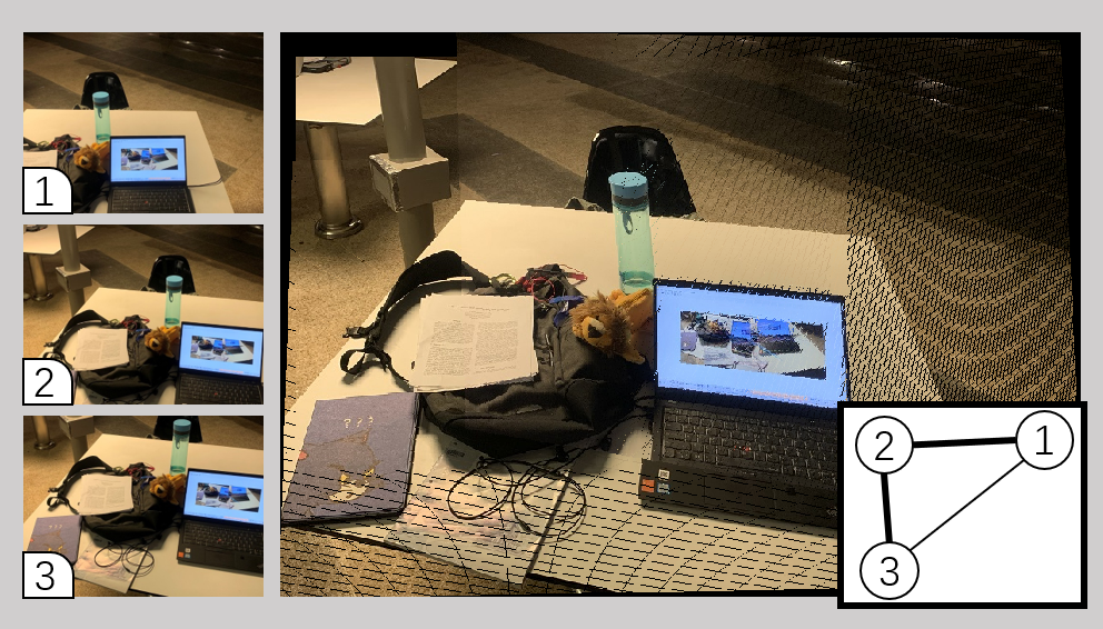
SIFT is an algorithm from the paper Distinctive Image Features from Scale-Invariant Keypoints, published by David G. Lowe in 2004. The solution for one of its application, image stitching, is proposed in Automatic Panoramic Image Stitching using Invariant Features, by Matthew Brown and David G. Lowe in 2017. The continuous assessment 1 of Visual Computing is based on these two papers.
3. Scale Invariant Feature Transform (SIFT) Algorithm
It’s the third feature detection algorithm introduced in the module EE5731. Here is an overview and the contents of the module: An Overview of EE5731 Visual Computing.
The paper Distinctive Image Features from Scale-Invariant Keypoints was first published in 1999 and attained perfection in 2004, by David Lowe from UBC. Although there is Scale-Invariant in its title, the features in SIFT are way more powerful than this. They are invariant to image rotation, illumination change, and partially invariant to 3D camera viewpoint.
The paper is well written, starting from theories and ending with a complete solution for object recognition. So instead of going through the whole paper, this post will only focus on introducing the framework, accompanying with useful notes when implementing this algorithm during the CA.
- Scale Space Extrema: Difference of Gaussian (DoG)
- Keypoint Localization: Taylor Expansion
- Contrast Threshold
- Edge Threshold
- Orientation Assignment
- Keypoint Descriptor
- Homography
- RANSAC
1 ~ 4 are the main steps covered in the paper. 5 and 6 are implemented along with SIFT in the assignment, which are covered in another paper, Automatic Panoramic Image Stitching using Invariant Features, from the same team.
3.1 Scale Space Extrema: Difference of Gaussian (DoG)
Input: an image
Output: the DoG and the locations of the scale space extrema in each DOG
When we think of selecting anchor points from an image, we prefer those stable ones, usually the extreme points or corners. It’s easy to find the extreme points that have larger pixel values than neighbouring pixels. But this will also include noise pixels and pixels on the edges, making the features unstable. Stable means the features points can be repeatably assigned under different views of the same object. Also, we hope the same object can give close feature descriptors to simplify the matching. The design of descriptors will be introduced later.
Scale space extrema are those extrema points coming from the difference-of-Gaussian (DoG) pyramids. Each pyramid is called an octave, which is formed by filtered images using Gaussian kernels. An octave of Gaussian filtered images can create difference-of-Gaussian images. Then we rescale the image, down-sample it by a factor of 2, and repeat the process.
For an image at a particular scale, is the convolution of a variable-scale Gaussian, :
The Gaussian blur in two dimensions is the product of two Gaussian functions:
Note that the formula of a Gaussian function in one dimension is:
The difference-of-Gaussian is:
The DoG function is a close approximation to the scale-normalized Laplacian of Gaussian (LoG) function. It’s proved that the extrema of LoG produces the most stable image features compared to a range of other possible image functions, such as the gradient, Hessian, or Harris corner function.
The maxima and minima of the difference-of-Gaussian images are then detected by comparing a pixel to its 26 neighbors at the current and adjacent scales (8 neighbors in the current image and 9 neighbors in the scale above and below).
3.2 Keypoint Localization: Taylor Expansion
Input: the locations of the scale space extrema from a DoG
Output: refined interpolated locations of the scale space extrema
Simply using the locations and the pixel values of the keypoints we get from 3.1 will not make the algorithm become invalid. However, the noise pixels will also give high response and be detected as keypoints in DoG.
The Taylor expansion with quadratic terms of is used to find out the location of the real extrema, (or , is the offset).
Let be the location of the keypoint in the DoG with variance , we have:
See Wikipedia for more help on vector multiplication. By setting , we have the extremum:
Since the computation only involves a 3x3 block around the keypoint candidate , we can copy the block and then set the center as original, . Then becomes the offset.
In case is larger than 0.5 on any dimension, it implies that the actual extremum is another pixel rather than . If so, we can set as the new center and fetch a new 3x3 block around it, repeat the calculation above till all the dimensions of are no larger than 0.5. With the final extremum, we can update the keypoints with the refined locations.
3.2.1 Contrast Threshold
Input: the refined location of a keypoint
Output: the contrast of the keypoint and the decision on whether it’s a noise pixel or not
The extremum location has another use in noise rejection. Most of the additional noise is not that strong. If the interpolated amplitude of the keypoint on DoG is less than 0.3, then it’s dropped out as a noise pixel.
Note that the image is normalized to from .
3.2.2 Edge Threshold
Input: the refined location of a keypoint
Output: whether it’s on a line or a vertex
Using the 3x3 block around the keypoint we can also compute a 2x2 matrix called Hessian matrix. The trace and determinant can be represented as the sum and the product of the 2 eigenvalues, and (say, ). They are also called principle curvatures. is the maximum curvature of the point and is the minimum curvature.
Let , then:
The empirical threshold is . If
, then is more likely that the keypoint lies on a line.
Consider the image as a 3D surface. The height of a point on it is the pixel value of . If the point lies on a line then it’s on a ridge or valley, making .
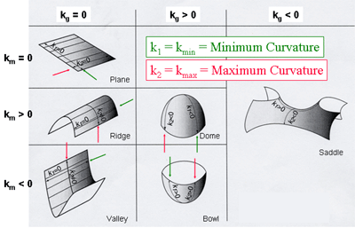
Figure 1
3.3 Orientation Assignment
Input: the image location, scale, and orientation of a keypoint
Output: an orientation histogram
3.4 Keypoint Descriptor
Input: the refined location of a keypoint
Output: a 4x4x8 = 128 element feature vector
All the steps above are from the paper Distinctive Image Features from Scale-Invariant Keypoints. The library VLFeat used in the CA is
3.5 Homography
Input: pairs of anchors in both images
Output: the homography matrix
Under construction
3.6 RANSAC
Input: all keypoints in both images
Output: the best pairs of keypoints to be the anchors
Under construction